Conclusion

If the result files of your model are satisfactory, you can then test your model on other data, especially your “test” folder.

But how do you know if your model is good? Open your results folder and let’s go through the important points to check:

• the mAP50-95 score:
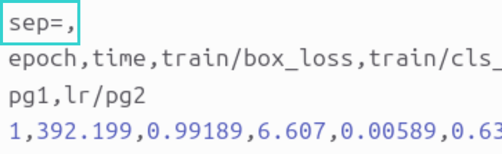
  • where to find it: in the results.csv file. Important point: in this file, the separator is a comma “,” whereas Excel expects semicolons, so the file may appear unreadable. To fix this issue, first open the file in a text editor and add a first line that says “sep=,” as shown in the image below:

• • save the modification, close the file, then open it in Excel.
  • each row corresponds to an epoch and each column contains values for different losses, metrics, and learning rate for that epoch. The column we are interested in is called: metrics/mAP50-95(B).
  • how to use it to evaluate your model: scroll all the way down to get the value of this metric at the last epoch of your model.
  • what is a good value:
    • below 0.3: bad
    • above 0.5: good for complex objects
    • above 0.7: excellent

• loss curves:
  • where to find them: in the results.png file to directly visualize the curves and their trends.
  • what to observe:
    • if both curves decrease and stabilize, your model is good
    • if the validation curves (val) increase while the training curves (train) decrease, your model is bad (sign of overfitting)

• F1 score curve:
  • where to find it: the file BoxF1_curve.png
  • what to check:
    • the curve should be as high as possible, close to 1.0.
  • what to extract:
    • take the x-value of the maximum, as it is the optimal confidence threshold. It is written in the legend next to “all classes” as: “all classes max_value at optimal_threshold”. You take the second value to use as the “conf” parameter when deploying your model.

• valbatchXpred.jpg images:
  • these images correspond to the model output, giving you a visual feedback of training. You can check whether detections are correct, bounding boxes are well placed, and no objects are missed.

If your model seems satisfactory, you can then test it on your “test” dataset folder to see how it performs. To do this, you must first load your trained model. It is usually located in runs/detect/trainx/weights and the file is best.pt:

from ultralytics import YOLO

model = YOLO("path/to/your/file/best.pt")

(feel free to use an absolute path unless you are on a cluster)

Then you can run a validation process, but making sure to specify that you want to use the test data. Don’t forget to add the test path in your data.yaml beforehand (it must be the same data.yaml used during training, otherwise create a new one like data_test.yaml and pass it as data=...).

metrics = model.val(split="test")

You will then find the results in runs/detect/valx, which you can analyze as explained earlier.

If these new results are also satisfactory, perfect. Otherwise, you will likely need to retrain your model. You may adjust some training parameters, but adding more epochs may be enough.

To continue training, start by loading the latest weights instead of the best ones (very important!), i.e. last.pt:

from ultralytics import YOLO

model = YOLO("path/to/your/file/last.pt")

Then start training as before, but with the parameter resume=True. Note that the number of epochs you specify is the total number of epochs, not additional ones. For example, if last.pt comes from 100 epochs, setting epochs=150 means you are adding 50 more epochs, not 150 additional ones.

results = model.train(epochs=150, resume=True)

Finally, if results are still not satisfactory, you may need to change some model parameters. This is covered in the next section.