Section outline
-
-
-
Once training is complete, you will be able to find your results in the “runs/detect/train” folder (unless you configured a different name for your results directory).
In this folder, you will find all the elements shown opposite (may vary):
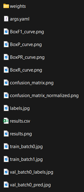 We will go through what each element represents one by one.
-
-
-
The “Weights” folder corresponds to the result of your work, as it contains the weights of your model. It is essentially your model stored in a file.
There are two files inside: “best.pt” and “last.pt”. This can be understood as follows: the weights of the neurons change continuously during training, and the quality of these weights is evaluated using a specific function. Therefore, last.pt corresponds to the most recent weights, while best.pt corresponds to the best weights obtained throughout the entire training process. We will discuss later why having two files can be useful.

-
-
-
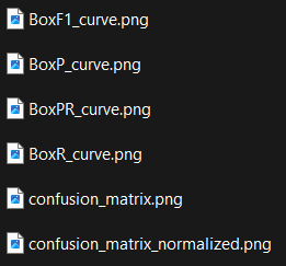
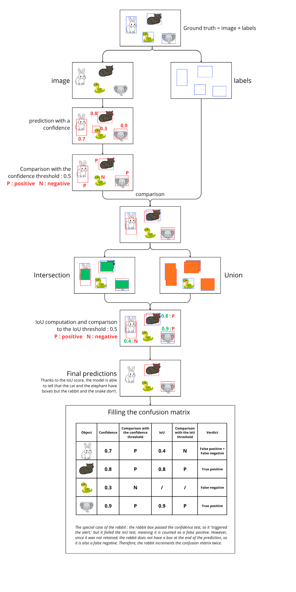
In computer vision, the “confusion matrix” is widely used, and it allows us to derive many relevant statistics to evaluate a model.
We need to go through a theoretical section before fully understanding what we are seeing, so you may need to focus a bit!
For this theoretical part, we will consider the case where we are trying to detect British coins called “pennies”.
Confusion Matrix
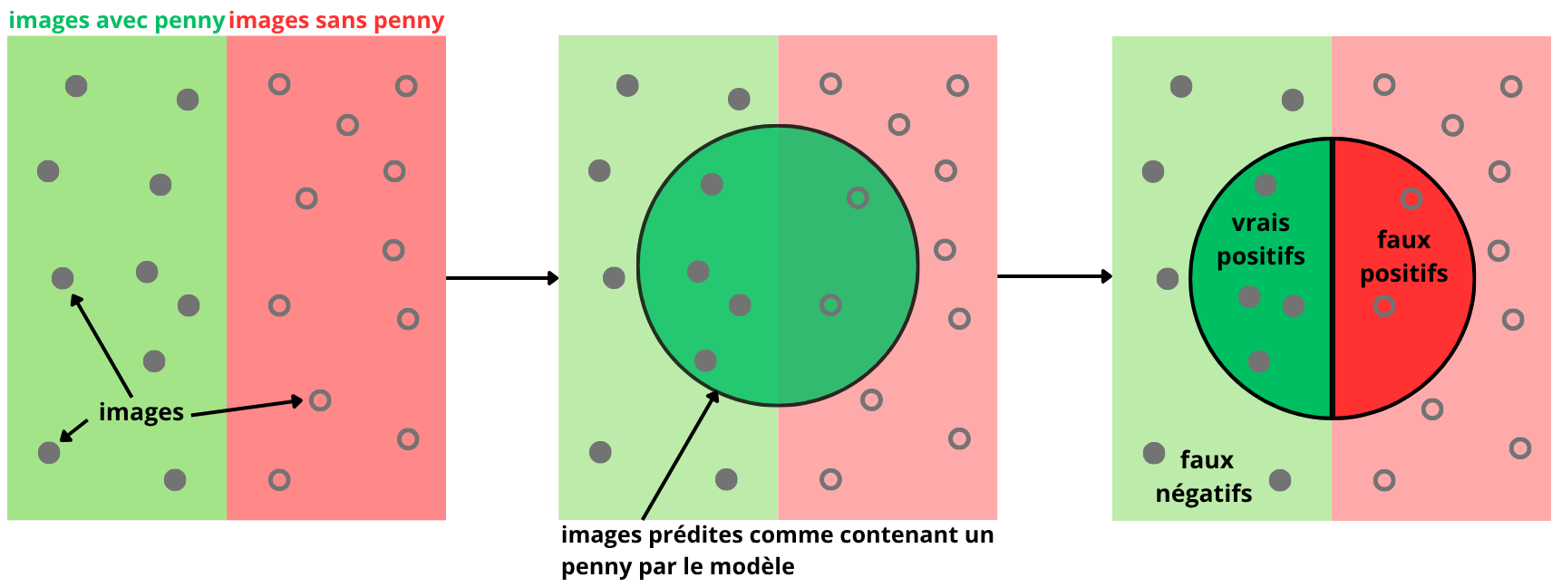
A confusion matrix is a table that summarizes and organizes the model’s predictions in order to analyze them.
For our example, we will use the following classes:
- “positive” corresponds to what we want to detect (we will use the “penny” class as an example)
- “negative” corresponds to the absence of the positive class (no “penny” present)
The rows correspond to the model’s predictions and the columns correspond to the ground truth.
To read a confusion matrix, you look at the intersection between a row and a column:
- w images predicted as positive (predicted to contain a “penny”) and actually positive (did contain a “penny”)
- and so on…
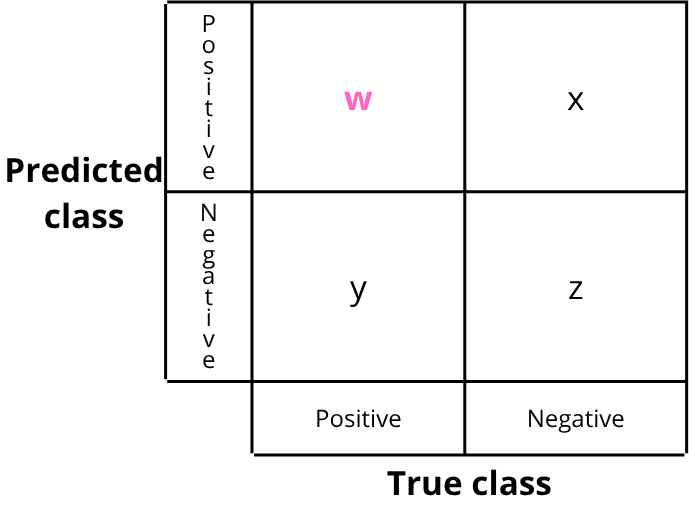
To make interpretation easier, names are given to the four cells:
- TP: True Positive
- What should be detected and is correctly detected.
- Example: a “penny” is present and correctly detected.
- TN: True Negative
- What should not be detected and is not detected.
- Example: no “penny” is present and none is detected.
- FP: False Positive
- What should be negative but is predicted as positive.
- Example: no “penny” is present but one is detected.
- FN: False Negative
- What should be positive but is predicted as negative.
- Example: a “penny” is present but not detected.
Example:
The image below corresponds to the ground truth, i.e., the manually annotated data that the model is expected to detect:
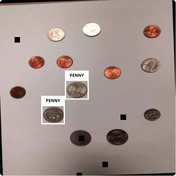
The next image corresponds to the detections made by the model on the same image after training:
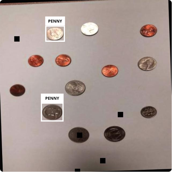
If we compare the two images:
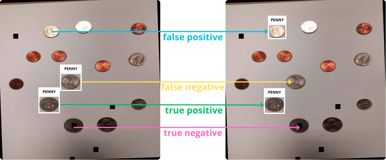
We then fill in the confusion matrix with each instance:
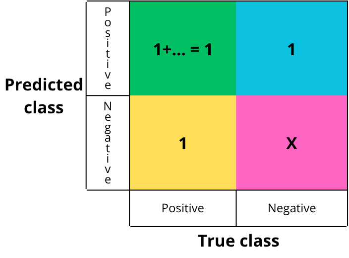
Each cell is filled by counting the number of occurrences of each event. In this simplified example, there is one of each. True negatives are not counted in detection tasks, as they are not meaningful: saying that nothing was detected when nothing was present becomes noise at the image scale.
From this matrix, we can derive several metrics to evaluate the model. Ultralytics provides four curves: precision-confidence, recall-confidence, precision-recall, and F1 score. We will see how to interpret them, but first let’s define each concept.
Confidence
When the model makes a prediction, it outputs a value representing the certainty of the prediction, i.e., a probability. This value, between 0 and 1, is called confidence (1 meaning absolute certainty).
A threshold value must be chosen. If the confidence is above this threshold, the detection is accepted (labeled “penny”); otherwise, it is rejected (labeled “background”/negative).
Example:
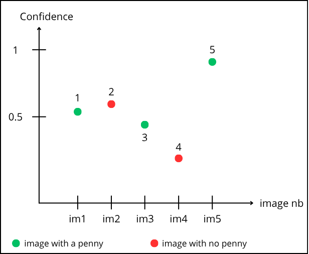
Reading the graph: point “1” corresponds to prediction on image 1. It is green, so a “penny” is present. The model predicts it with a confidence of 0.55.
Point “2” corresponds to image 2. It is red (no “penny”), but the model predicts a “penny” with 0.6 confidence.
Let’s choose a threshold of 0.5. Points above are accepted, below are rejected :
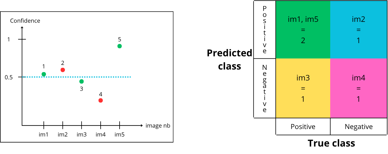
How to fill the matrix:
-
Point “1” is above the confidence threshold, so it is predicted positive (contains a penny) and is green (actually contains a penny) → True Positive
-
Point “2” is above the confidence threshold, so it is predicted positive (contains a penny) and is red (does not contain a penny) → False Positive
-
Point “3” is below the confidence threshold, so it is predicted negative (does not contain a penny) and is green (actually contains a penny) → False Negative
-
Point “4” is below the confidence threshold, so it is predicted negative (does not contain a penny) and is red (does not contain a penny) → True Negative
-
Point “5” is above the confidence threshold, so it is predicted positive (contains a penny) and is green (actually contains a penny) → True Positive
Now let’s try a threshold of 0.75:

-
Point “1” is below the threshold, so it is predicted negative but green → False Negative
-
Point “2” is below the threshold, so it is predicted negative and red → True Negative
-
Point “3” is below the threshold, so it is predicted negative but green → False Negative
-
Point “4” is below the threshold, so it is predicted negative and red → True Negative
-
Point “5” is above the threshold, so it is predicted positive and green → True Positive
Finally, let’s try a threshold of 0.35:
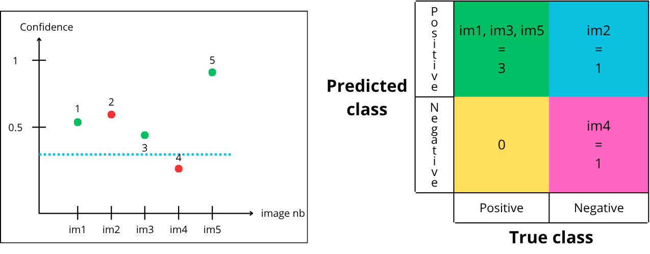
- Point “1” is above the threshold, so it is predicted positive and is green → True Positive
- Point “2” is above the threshold, so it is predicted positive but is red → False Positive
- Point “3” is above the threshold, so it is predicted positive and is green → True Positive
- Point “4” is below the threshold, so it is predicted negative and is red → True Negative
- Point “5” is above the threshold, so it is predicted positive and is green → True Positive
Now it’s your turn — a short exercise:
For a given model, there are multiple possible confusion matrices, depending on the chosen confidence threshold :
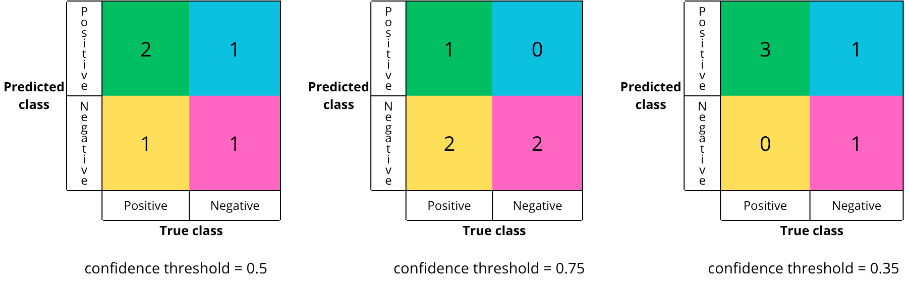
In theory, there are an infinite number of confusion matrices, as there are an infinite number of threshold values between 0 and 1.
The confusion matrix reflects the quality of the chosen confidence threshold. One key objective after training is to select the best threshold for deployment.
But how to know if a confusion matrix is a good one. A good matrix maximizes the correct diagonal (true positives and true negatives) and minimizes the bad diagonal (false positives and falses negatives).
However, in practice, reducing both errors simultaneously is difficult, so trade-offs must be made. For example, in medicine, false negatives are minimized (to avoid missing a disease), even if it increases false positives.
To determine the best threshold, we rely on evaluation metrics which we gonna see in the next section.
-
-
-
Let’s visualize these metrics using a diagram:
Using the previous diagram, we can express precision and recall as follows:
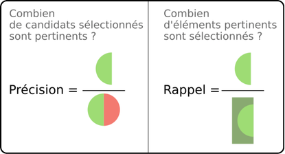
Mathematically, this can be formalized as follows:


It is therefore possible to plot curves to observe how these metrics evolve as a function of the confidence threshold.
Precision–Confidence
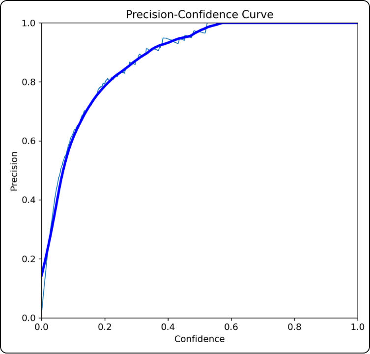
How is it constructed? For all confidence thresholds between 0 and 1:
- compute the confusion matrix for that threshold
- compute the precision associated with this specific matrix
- plot the point on the graph
How should it be interpreted? For example, at a confidence threshold of 0.4, the precision is around 0.92. This indicates that at this threshold, there are relatively few false positives.
Key takeaway: the higher the curve, the better the model.
Further insight:
This curve must be interpreted carefully because it does not account for false negatives. Moreover, as the threshold increases, fewer predictions are considered, so the increase in precision can be somewhat “artificial”.
This happens because the model becomes very selective. For example, if it only detects one true positive with 98% confidence, it will achieve 100% precision, even though many true positives (below the threshold) are missed.
Recall–Confidence
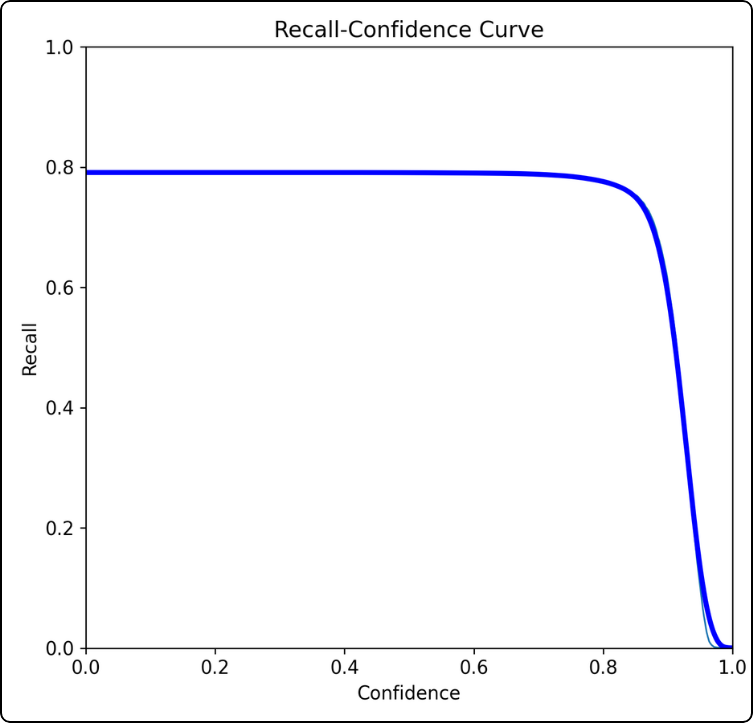
How is it constructed? For all confidence thresholds between 0 and 1:
- compute the confusion matrix for that threshold
- compute the recall associated with this specific matrix
- plot the point on the graph
How should it be interpreted? For example, at a confidence threshold of 0.8, the recall is around 0.78. This indicates that at this threshold, there are many false negatives.
Key takeaway: the higher the curve and the longer it takes to drop, the better the model.
Further insight:
The curve will inevitably reach 0 because as the confidence threshold increases, the model becomes stricter and accepts fewer predictions. This leads to a sharp increase in false negatives, which drives the recall down.
Precision and recall are both useful metrics but they are complementary. To properly evaluate a model, both must be considered together, especially how one evolves relative to the other.
To avoid constantly switching between the two graphs, combined metrics are used. We will therefore introduce the precision–recall curve and the F1-score in the next section.
-
-
-
The precision-recall curve shows the simultaneous evolution of precision and recall depending on the confidence threshold. It is built in a very specific way, which we will explain just after.
The F1-score is the harmonic mean of precision and recall. This curve is used to find the optimal confidence threshold for deploying your model.
-
-
-
-
Precision-Recall
-
-
-
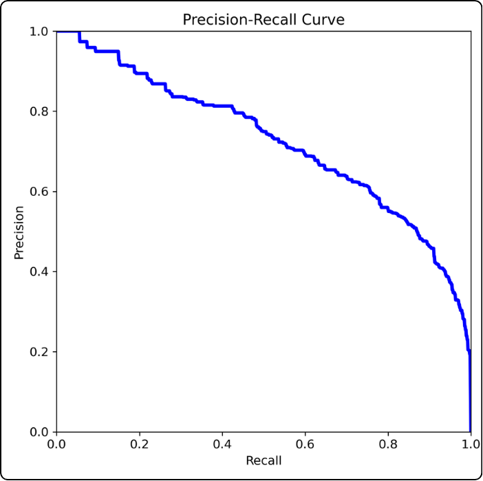
How to build it? This curve is constructed point by point because a third dimension is hidden: the confidence threshold.
We start with the leftmost point: this point corresponds to the precision and recall values when the confidence threshold is 1.
Then we plot the next point to the right: we take a threshold of 0.99 and compute precision and recall from the confusion matrix. And so on.
How to read it? For example, consider the point where the confidence threshold is 0.5 (if you stretch the curve between your fingers, this would be the middle). At this threshold, we can read a precision of about 0.65 and a recall of about 0.67.
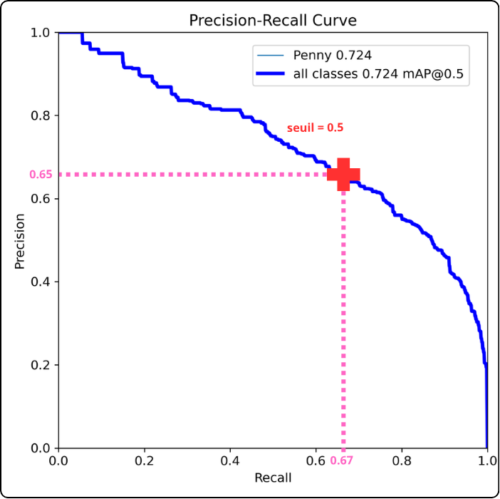
Key takeaway: the closer the curve gets to the top-right corner, the better the model performs (this example model is actually quite poor, so don’t rely on it).
Going further:
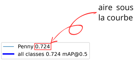
The precision-recall curve is used to compute another metric that you will encounter in the results: Average Precision (AP). This metric corresponds to the area under the precision-recall curve. It is the decimal value shown next to each class name in the legend.
By extension, mAP stands for mean Average Precision, which is the average of AP values when multiple classes are involved.
Why is this useful? As mentioned earlier, “getting closer to the top-right corner” is subjective. AP was introduced to quantify how high the curve rises, i.e., how large the area under the curve is. The higher the AP or mAP, the better the model.
Going even further:
After “mAP”, you may see “@0.5”, which corresponds to the threshold value for Intersection over Union (IoU).
To understand IoU, think of it as a verification tool for the model: the model predicts a bounding box, and there is also a ground-truth bounding box. We need a way to quantify how well the predicted box matches the true one.
Consider the two boxes below:

The green box represents ground truth, and the orange box is the model’s prediction. It is not perfectly placed, but it still roughly covers the same object.
To measure this, we compute the ratio between the intersection and the union of the two boxes, as illustrated below:
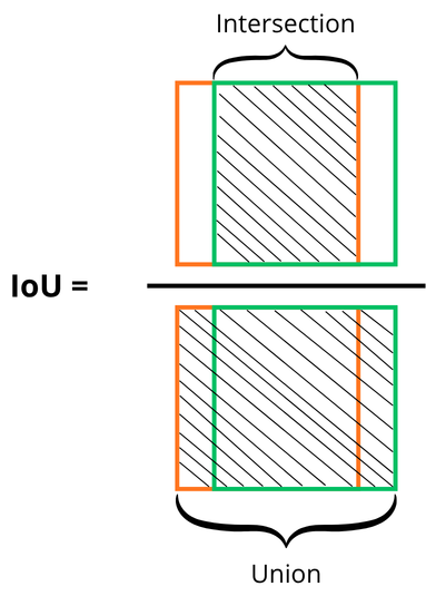
A threshold must be chosen to accept or reject predictions. For example, with an IoU threshold of 0.5, a predicted box must overlap the ground-truth box by at least 50% to be considered valid.
What is the difference between confidence and IoU?
Step 1: choose thresholds (arbitrarily):
- confidence threshold = 0.5
- IoU threshold = 0.5
Step 2: the model trains, processes images, and produces predictions with associated confidence scores.
Step 3: based on the confidence threshold, the model accepts predictions above the threshold and rejects the others.
Step 4: verification phase. Predicted boxes are compared to ground-truth boxes using IoU:
- If IoU ≥ threshold → true positive
- If IoU < threshold but passed confidence → false positive
Step 5: ground-truth boxes with no matching prediction are counted as false negatives.
The key difference is that the IoU threshold is only used during training, whereas the confidence threshold is crucial during deployment.
The diagram below explains what si going on with an image :
Another metric you may encounter is mAP50-95. It computes mAP across IoU thresholds from 0.5 to 0.95 (step 0.05) and takes the average.
This metric is particularly useful because it is stricter about bounding-box accuracy, making it a standard benchmark in computer vision.
-
-
-
-
F1-score
-
-
-
The F1-score is the harmonic mean of precision and recall:

One key advantage of F1 is its sensitivity to extreme values. A model with perfect precision but very low recall will still get a poor F1 score.
This curve is used to find the optimal confidence threshold: it corresponds to the x-value of the maximum point on the curve.
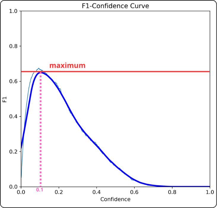
Key takeaway: the x-value at the maximum is a good candidate for your confidence threshold.
If the F1 curve forms a plateau instead of a sharp peak:
- Prioritize precision (avoid false positives): choose the right end of the plateau (higher threshold).
- Prioritize recall (avoid false negatives): choose the left end (lower threshold).
- Balanced approach: choose the center of the plateau.
-
-
-
-
What is multi-class? It is when you have more than one class to detect, for example you have penny, dime and nickel (three different types of coins).
In your confusion matrix, you will therefore have as many rows and columns as classes, to which we add the “negative” (”background”) row and column that corresponds to the absence of a class.
Let’s see what it looks like:
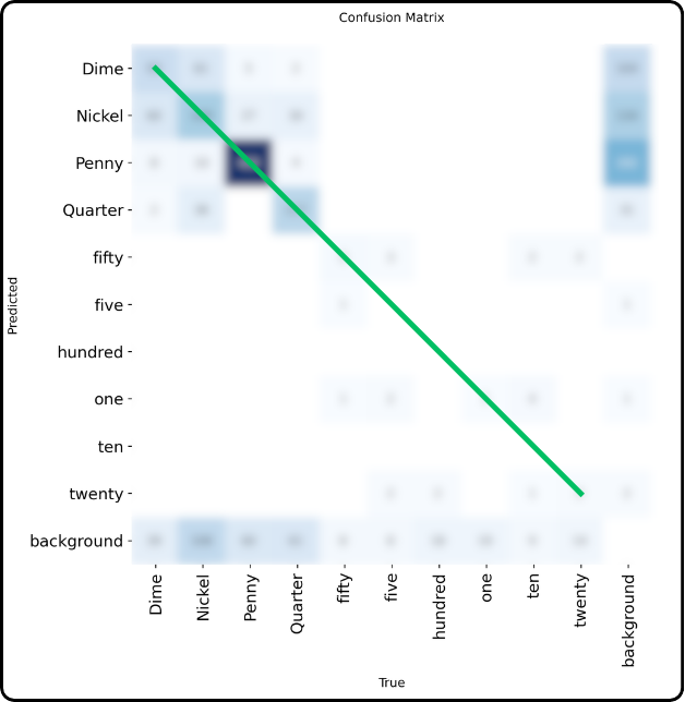
The rows correspond to predictions and the columns to ground truth for each class.
We clearly find the correct diagonal which still corresponds to cases where the predicted class matches the ground truth.
However, there is no longer a wrong diagonal. Incorrect predictions now occupy all other cells in the matrix.
The far-right column corresponds to objects that were detected but actually belong to the background. Conversely, the last row corresponds to objects that were not detected but actually belonged to a class.
With this new confusion matrix format, it becomes necessary to define what are true positives, true negatives, false positives, and false negatives. This will allow us to compute precision, recall, and F1-score in order to find the best confidence threshold for deploying the model.
To reduce a multi-class matrix to a 2x2 matrix, we proceed class by class. In the end, we will have as many 2x2 confusion matrices as there are classes (excluding "background").
To fill them, let’s see how to determine what corresponds to what.
First, we do not need true negatives as seen earlier.
Let’s see how to find the remaining three using the “Penny” class as an example.
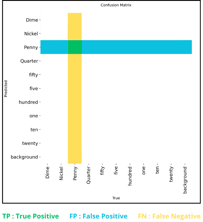
The true positives are those predicted as “penny” that were indeed pennies, so there is only one cell: the green one at the intersection of the "penny" row and "penny" column.
Next, the cells in the same row correspond to objects predicted as “penny” but which were not, i.e., false positives.
Finally, the cells in the same column correspond to objects predicted as anything except “penny” but which were actually pennies, i.e., false negatives.
For false negatives and false positives, we sum the values of all the corresponding cells.
Once we have our 3 values (TP, TN, FP), we can compute precision and recall, and then derive the precision-recall and F1-score curves. As seen previously, we repeat this process for all confidence thresholds to plot the curves.
Then, once the curves for one class are drawn, we repeat for the next class, and so on, until all are computed. We end up with as many curves as classes.
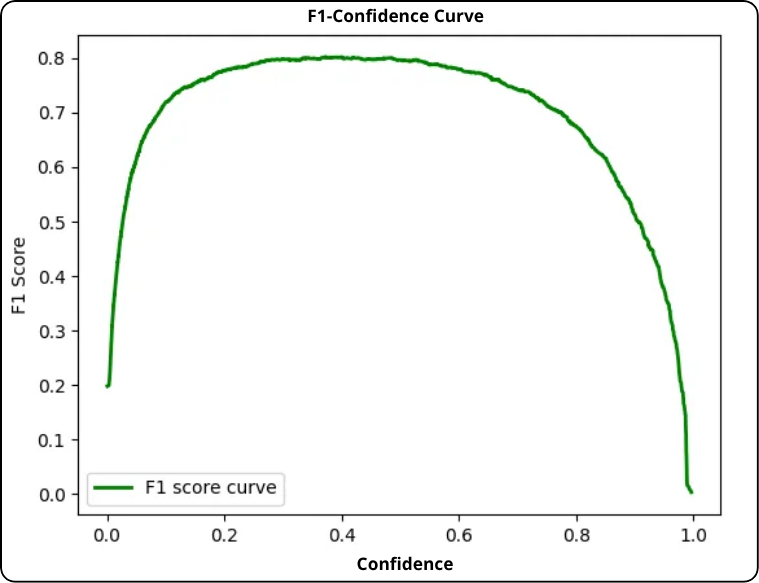
To get an overall view, we take the average of all these curves, which corresponds to the bold curve shown in the F1-score graph below.
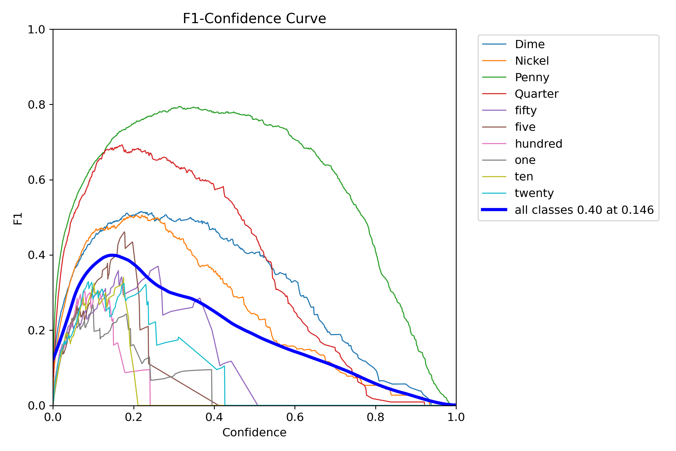
And the “0.40 at 0.146” next to “all classes” corresponds to the peak of the curve: the maximum is 0.40 and its x-value is 0.146, so in this experiment, a confidence threshold of 0.146 should be chosen.
-
-
Normalized multi-class confusion matrix
-
Finally, there is the normalized confusion matrix. It provides an overall view because instead of raw counts, it shows percentages.
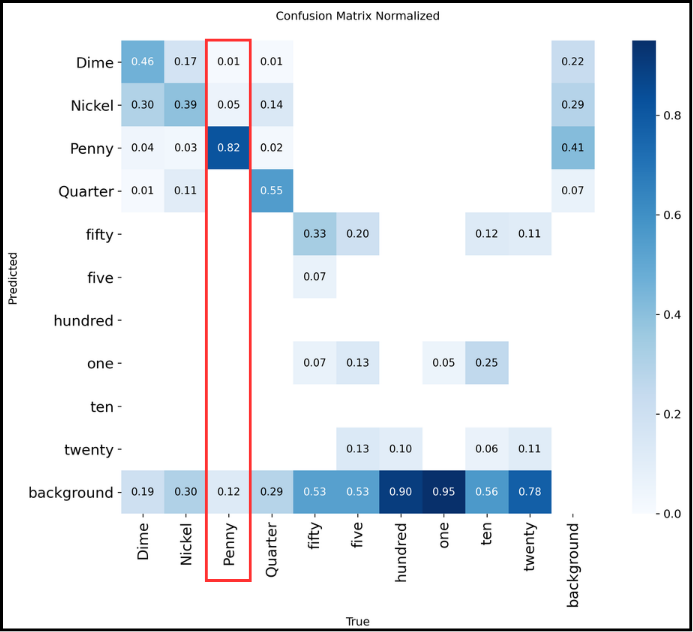
How to read it?
The normalized confusion matrix shows detection percentages for each class, so it is read column by column. For example, for “Penny” from top to bottom:
- 1% were predicted as “Dime”
- 5% were confused with “Nickel”
- 82% of “Penny” were correctly recognized
- 12% were not detected at all
The total sums to 100%, so everything is consistent.
-
-
-
-
labels.jpg is an image containing four plots similar to the one below:
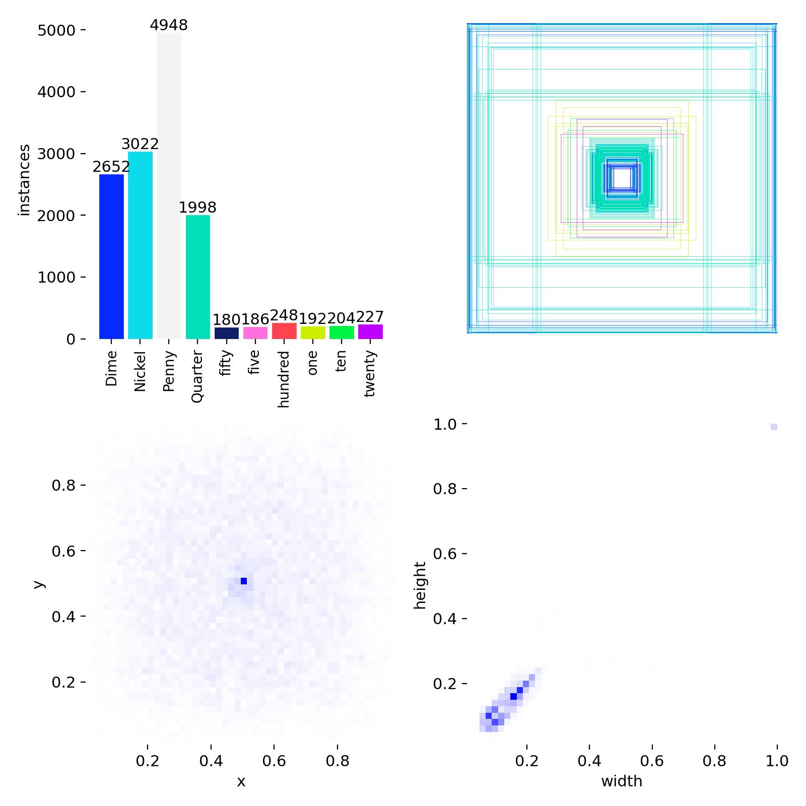
Top left: distribution of the different classes.
Top right: overlay of all bounding boxes.
Bottom left: coordinates of the centers of the bounding boxes.
Bottom right: dimensions of the bounding boxes.
These are statistics about the annotated data; this file is independent of training.
-
-
-
These documents contain the same metrics, one in CSV table form, the other in graphical form.
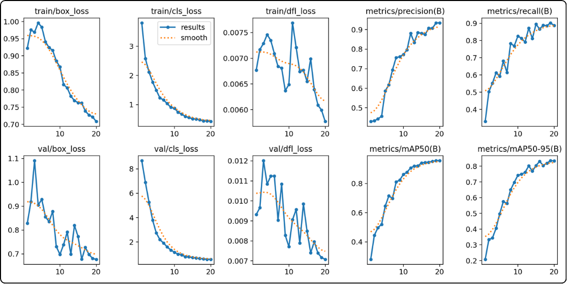
- The six curves on the left (the losses) : the model is learning and making fewer errors
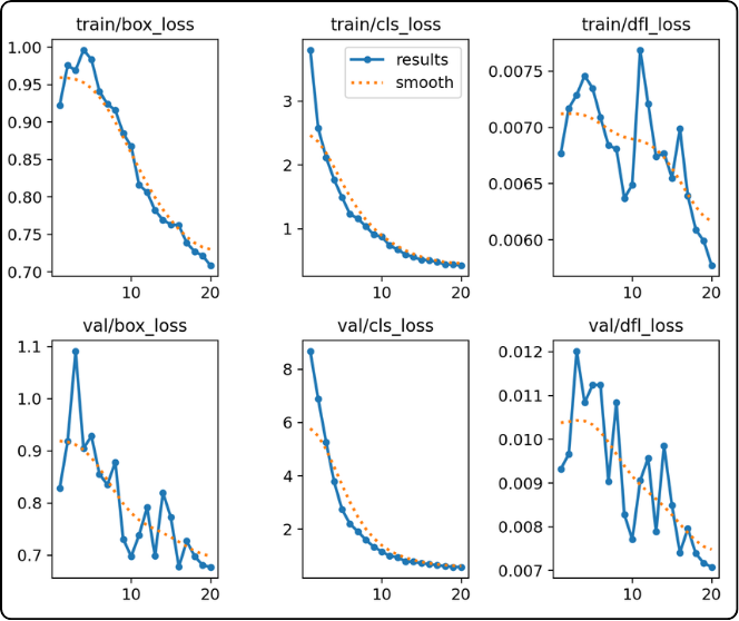
These 6 curves correspond to the error between predictions and ground truth, with training on the top and validation on the bottom.
During training, there is a phenomenon to be careful about: overfitting. Simply put, it means the model is learning the training data by heart.
Why is this a problem? Because the model will no longer generalize well to different data, even if it is similar.
How can we tell if the model is overfitting? This can be seen using the validation data, since the model does not train on it; it only uses it for evaluation.
So when looking at the loss curves, if the training curves (top) continue to decrease while the validation curves (bottom) start increasing at some point, it is a sign of overfitting because validation losses begin to rise again.
In the example above, we can see that the validation curves keep decreasing, which indicates that the model is currently generalizing well.
If overfitting occurs, what are the consequences?
As mentioned earlier, YOLO saves two models: best.pt and last.pt. In last.pt, you will find the overfitted model. However, in best.pt, YOLO stores the weights that achieved the best combined performance on training and validation, i.e., before overfitting occurs.
So if best.pt already contains weights from before overfitting, what is the problem of overfitting? It can be seen as a waste of computational resources, since the model goes too far. To address this, we can use the “patience” parameter, which tells the model: “if after x epochs the model does not improve anymore (i.e., best.pt weights do not change), then stop training”, where x is a positive integer.
- The four curves on the right (precision, recall, mAP50, mAP50-95) : the model becomes more performant
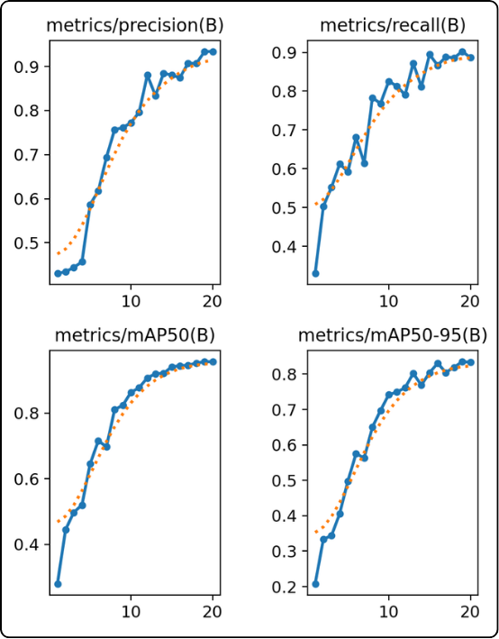
They allow us to see whether the model has reached its full potential.
These curves help visualize whether the model is improving. A good indicator that the model is reaching its final state is when these curves reach a plateau. In that case, we know the model has reached its best performance and has no further improvement potential.
For example, in the case above, we can see that after 20 epochs, the curves are still increasing, which indicates that the model would need more epochs to stabilize.
-
-
-
If the result files of your model are satisfactory, you can then test your model on other data, especially your “test” folder.
But how do you know if your model is good? Open your results folder and let’s go through the important points to check:
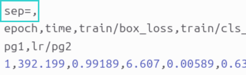
- the mAP50-95 score:
- where to find it: in the results.csv file. Important point: in this file, the separator is a comma “,” whereas Excel expects semicolons, so the file may appear unreadable. To fix this issue, first open the file in a text editor and add a first line that says “sep=,” as shown in the image below:
-
- save the modification, close the file, then open it in Excel.
- each row corresponds to an epoch and each column contains values for different losses, metrics, and learning rate for that epoch. The column we are interested in is called: metrics/mAP50-95(B).
- how to use it to evaluate your model: scroll all the way down to get the value of this metric at the last epoch of your model.
- what is a good value:
- below 0.3: bad
- above 0.5: good for complex objects
- above 0.7: excellent
- loss curves:
- where to find them: in the results.png file to directly visualize the curves and their trends.
- what to observe:
- if both curves decrease and stabilize, your model is good
- if the validation curves (val) increase while the training curves (train) decrease, your model is bad (sign of overfitting)
- F1 score curve:
- where to find it: the file BoxF1_curve.png
- what to check:
- the curve should be as high as possible, close to 1.0.
- what to extract:
- take the x-value of the maximum, as it is the optimal confidence threshold. It is written in the legend next to “all classes” as: “all classes max_value at optimal_threshold”. You take the second value to use as the “conf” parameter when deploying your model.
- valbatchXpred.jpg images:
- these images correspond to the model output, giving you a visual feedback of training. You can check whether detections are correct, bounding boxes are well placed, and no objects are missed.
If your model seems satisfactory, you can then test it on your “test” dataset folder to see how it performs. To do this, you must first load your trained model. It is usually located in runs/detect/trainx/weights and the file is best.pt:
from ultralytics import YOLOmodel = YOLO("path/to/your/file/best.pt")(feel free to use an absolute path unless you are on a cluster)
Then you can run a validation process, but making sure to specify that you want to use the test data. Don’t forget to add the test path in your data.yaml beforehand (it must be the same data.yaml used during training, otherwise create a new one like data_test.yaml and pass it as data=...).
metrics = model.val(split="test")You will then find the results in runs/detect/valx, which you can analyze as explained earlier.
If these new results are also satisfactory, perfect. Otherwise, you will likely need to retrain your model. You may adjust some training parameters, but adding more epochs may be enough.
To continue training, start by loading the latest weights instead of the best ones (very important!), i.e. last.pt:
from ultralytics import YOLOmodel = YOLO("path/to/your/file/last.pt")Then start training as before, but with the parameter resume=True. Note that the number of epochs you specify is the total number of epochs, not additional ones. For example, if last.pt comes from 100 epochs, setting epochs=150 means you are adding 50 more epochs, not 150 additional ones.
results = model.train(epochs=150, resume=True)Finally, if results are still not satisfactory, you may need to change some model parameters. This is covered in the next section.
- the mAP50-95 score:
-
-