confusion_matrix.png - confusion_matrix_normalized.png

What is multi-class? It is when you have more than one class to detect, for example you have penny, dime and nickel (three different types of coins).

In your confusion matrix, you will therefore have as many rows and columns as classes, to which we add the “negative” (”background”) row and column that corresponds to the absence of a class.

Let’s see what it looks like:

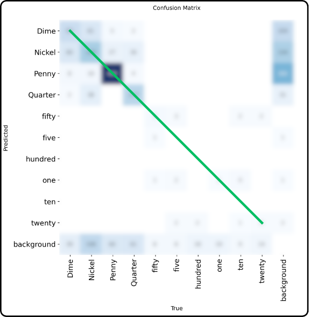
The rows correspond to predictions and the columns to ground truth for each class.

We clearly find the correct diagonal which still corresponds to cases where the predicted class matches the ground truth.

However, there is no longer a wrong diagonal. Incorrect predictions now occupy all other cells in the matrix.

The far-right column corresponds to objects that were detected but actually belong to the background. Conversely, the last row corresponds to objects that were not detected but actually belonged to a class.

With this new confusion matrix format, it becomes necessary to define what are true positives, true negatives, false positives, and false negatives. This will allow us to compute precision, recall, and F1-score in order to find the best confidence threshold for deploying the model.

To reduce a multi-class matrix to a 2x2 matrix, we proceed class by class. In the end, we will have as many 2x2 confusion matrices as there are classes (excluding "background").

To fill them, let’s see how to determine what corresponds to what.

First, we do not need true negatives as seen earlier.

Let’s see how to find the remaining three using the “Penny” class as an example.

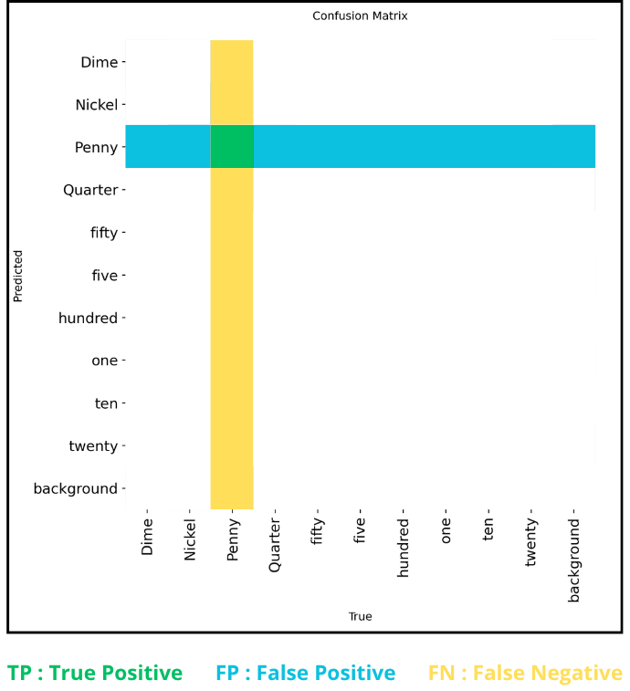
The true positives are those predicted as “penny” that were indeed pennies, so there is only one cell: the green one at the intersection of the "penny" row and "penny" column.

Next, the cells in the same row correspond to objects predicted as “penny” but which were not, i.e., false positives.

Finally, the cells in the same column correspond to objects predicted as anything except “penny” but which were actually pennies, i.e., false negatives.

For false negatives and false positives, we sum the values of all the corresponding cells.

Once we have our 3 values (TP, TN, FP), we can compute precision and recall, and then derive the precision-recall and F1-score curves. As seen previously, we repeat this process for all confidence thresholds to plot the curves.

Then, once the curves for one class are drawn, we repeat for the next class, and so on, until all are computed. We end up with as many curves as classes.

To get an overall view, we take the average of all these curves, which corresponds to the bold curve shown in the F1-score graph below.

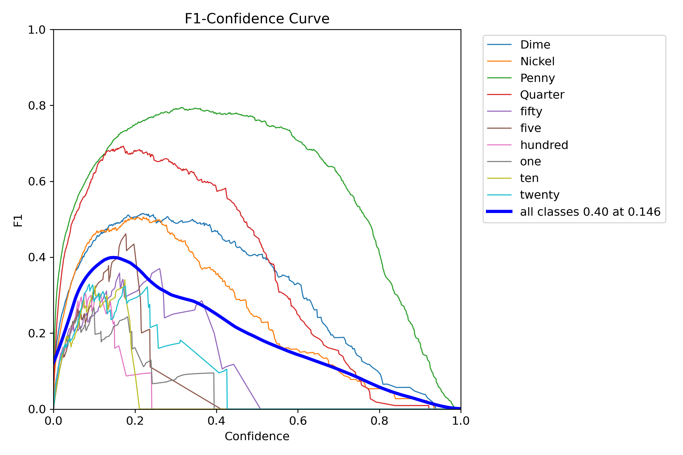
And the “0.40 at 0.146” next to “all classes” corresponds to the peak of the curve: the maximum is 0.40 and its x-value is 0.146, so in this experiment, a confidence threshold of 0.146 should be chosen.

• • Normalized multi-class confusion matrix

Finally, there is the normalized confusion matrix. It provides an overall view because instead of raw counts, it shows percentages.

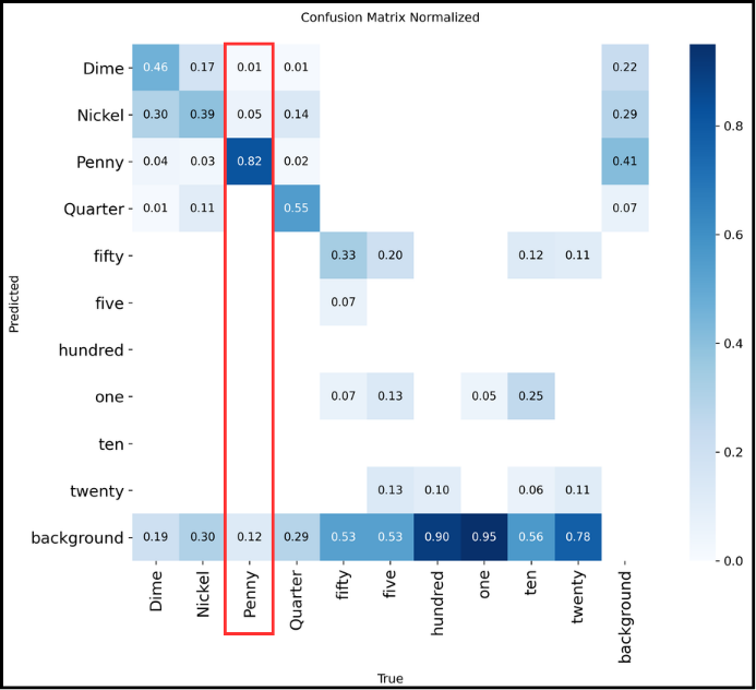
How to read it?

The normalized confusion matrix shows detection percentages for each class, so it is read column by column. For example, for “Penny” from top to bottom:

• 1% were predicted as “Dime”
• 5% were confused with “Nickel”
• 82% of “Penny” were correctly recognized
• 12% were not detected at all

The total sums to 100%, so everything is consistent.