Section outline
-
In computer vision, the “confusion matrix” is widely used, and it allows us to derive many relevant statistics to evaluate a model.
We need to go through a theoretical section before fully understanding what we are seeing, so you may need to focus a bit!
For this theoretical part, we will consider the case where we are trying to detect British coins called “pennies”.
Confusion Matrix
A confusion matrix is a table that summarizes and organizes the model’s predictions in order to analyze them.
For our example, we will use the following classes:
- “positive” corresponds to what we want to detect (we will use the “penny” class as an example)
- “negative” corresponds to the absence of the positive class (no “penny” present)
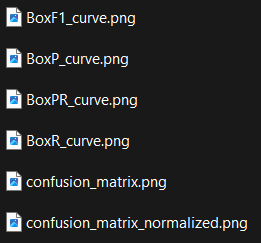
The rows correspond to the model’s predictions and the columns correspond to the ground truth.
To read a confusion matrix, you look at the intersection between a row and a column:
- w images predicted as positive (predicted to contain a “penny”) and actually positive (did contain a “penny”)
- and so on…
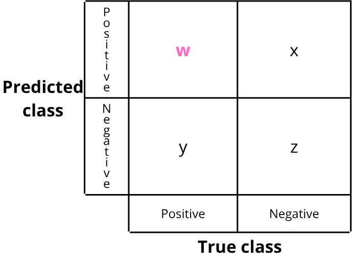
To make interpretation easier, names are given to the four cells:
- TP: True Positive
- What should be detected and is correctly detected.
- Example: a “penny” is present and correctly detected.
- TN: True Negative
- What should not be detected and is not detected.
- Example: no “penny” is present and none is detected.
- FP: False Positive
- What should be negative but is predicted as positive.
- Example: no “penny” is present but one is detected.
- FN: False Negative
- What should be positive but is predicted as negative.
- Example: a “penny” is present but not detected.
Example:
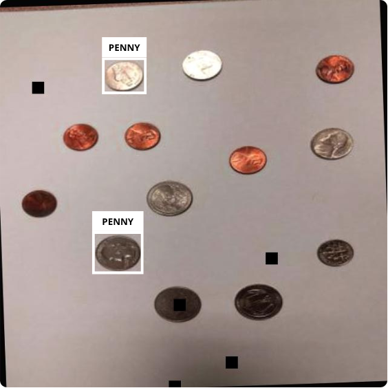
The image below corresponds to the ground truth, i.e., the manually annotated data that the model is expected to detect:
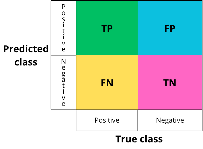
The next image corresponds to the detections made by the model on the same image after training:
If we compare the two images:
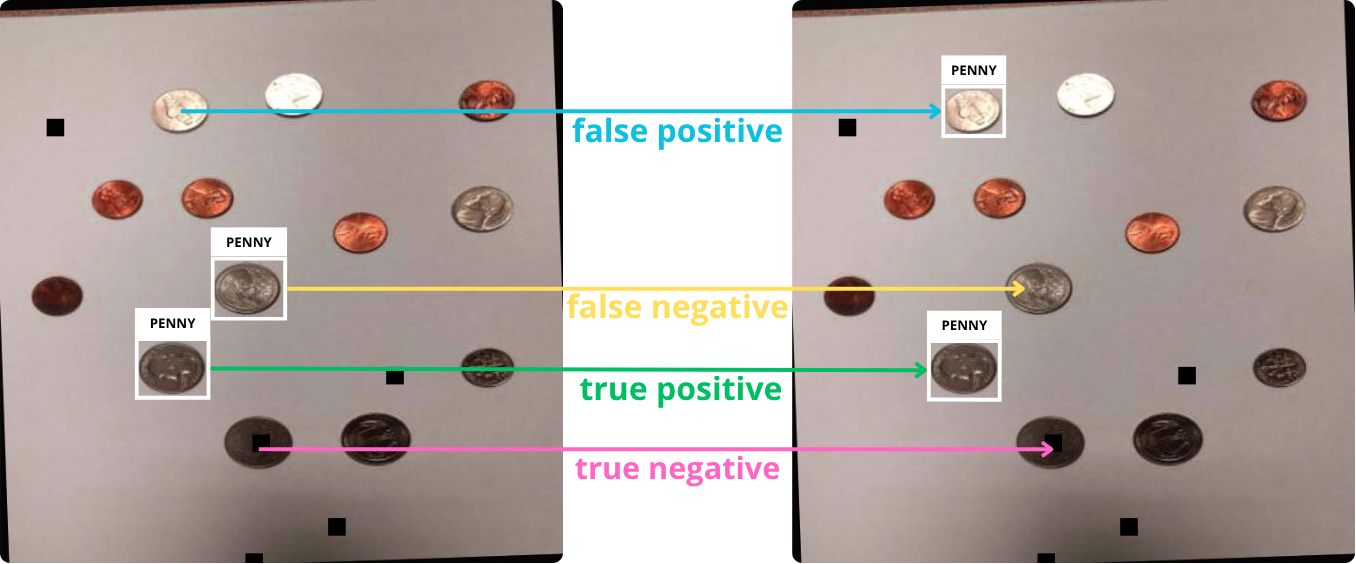
We then fill in the confusion matrix with each instance:
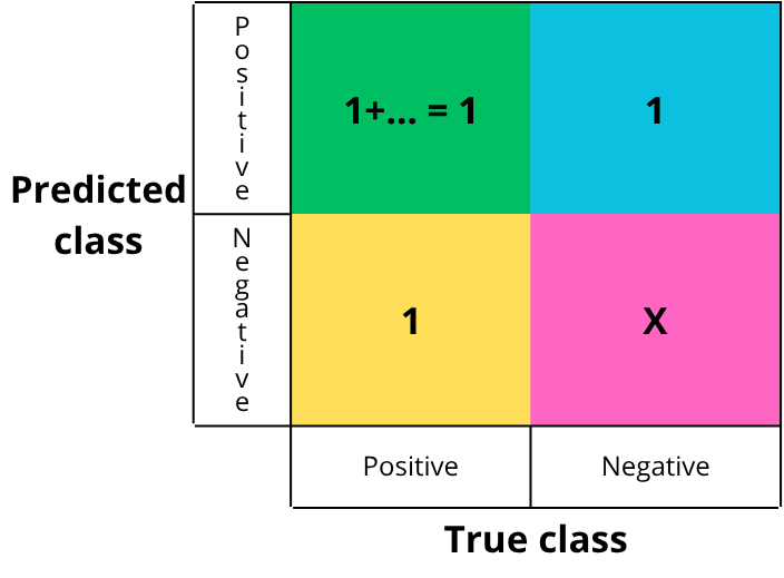
Each cell is filled by counting the number of occurrences of each event. In this simplified example, there is one of each. True negatives are not counted in detection tasks, as they are not meaningful: saying that nothing was detected when nothing was present becomes noise at the image scale.
From this matrix, we can derive several metrics to evaluate the model. Ultralytics provides four curves: precision-confidence, recall-confidence, precision-recall, and F1 score. We will see how to interpret them, but first let’s define each concept.
Confidence
When the model makes a prediction, it outputs a value representing the certainty of the prediction, i.e., a probability. This value, between 0 and 1, is called confidence (1 meaning absolute certainty).
A threshold value must be chosen. If the confidence is above this threshold, the detection is accepted (labeled “penny”); otherwise, it is rejected (labeled “background”/negative).
Example:
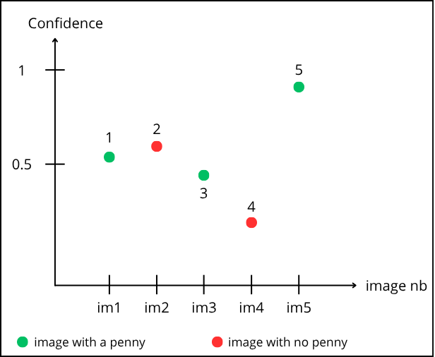
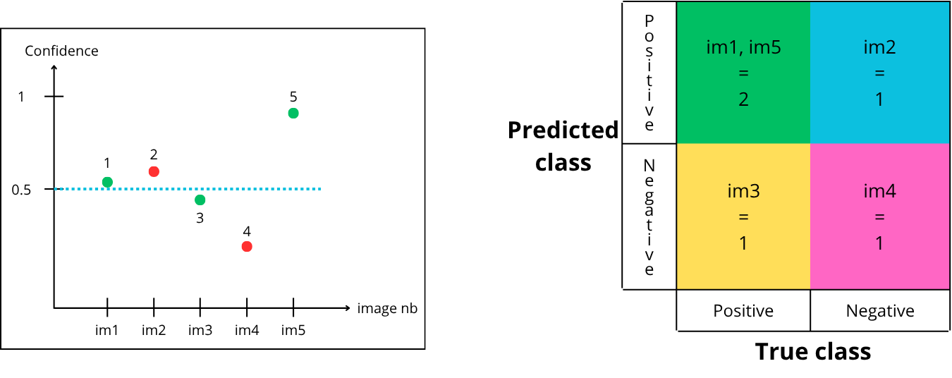
Reading the graph: point “1” corresponds to prediction on image 1. It is green, so a “penny” is present. The model predicts it with a confidence of 0.55.
Point “2” corresponds to image 2. It is red (no “penny”), but the model predicts a “penny” with 0.6 confidence.
Let’s choose a threshold of 0.5. Points above are accepted, below are rejected :
How to fill the matrix:
-
Point “1” is above the confidence threshold, so it is predicted positive (contains a penny) and is green (actually contains a penny) → True Positive
-
Point “2” is above the confidence threshold, so it is predicted positive (contains a penny) and is red (does not contain a penny) → False Positive
-
Point “3” is below the confidence threshold, so it is predicted negative (does not contain a penny) and is green (actually contains a penny) → False Negative
-
Point “4” is below the confidence threshold, so it is predicted negative (does not contain a penny) and is red (does not contain a penny) → True Negative
-
Point “5” is above the confidence threshold, so it is predicted positive (contains a penny) and is green (actually contains a penny) → True Positive
Now let’s try a threshold of 0.75:

-
Point “1” is below the threshold, so it is predicted negative but green → False Negative
-
Point “2” is below the threshold, so it is predicted negative and red → True Negative
-
Point “3” is below the threshold, so it is predicted negative but green → False Negative
-
Point “4” is below the threshold, so it is predicted negative and red → True Negative
-
Point “5” is above the threshold, so it is predicted positive and green → True Positive
Finally, let’s try a threshold of 0.35:
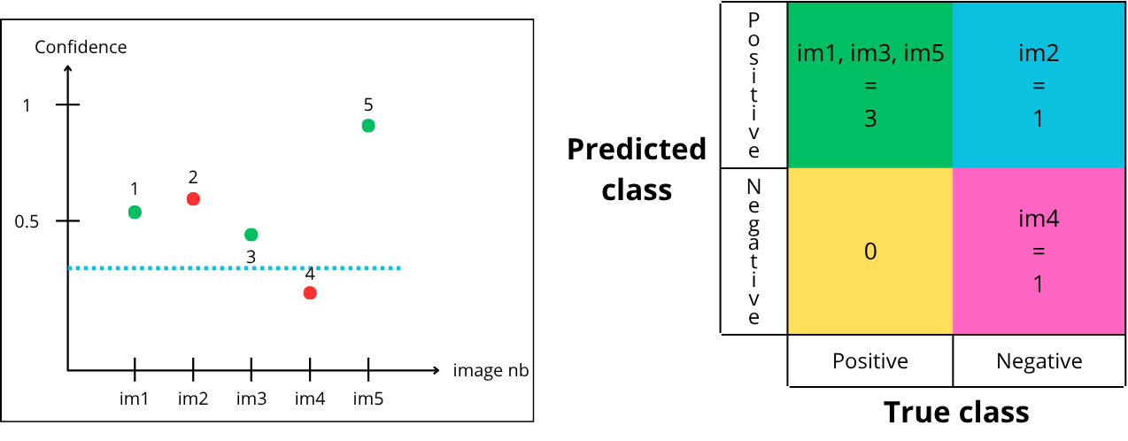
- Point “1” is above the threshold, so it is predicted positive and is green → True Positive
- Point “2” is above the threshold, so it is predicted positive but is red → False Positive
- Point “3” is above the threshold, so it is predicted positive and is green → True Positive
- Point “4” is below the threshold, so it is predicted negative and is red → True Negative
- Point “5” is above the threshold, so it is predicted positive and is green → True Positive
Now it’s your turn — a short exercise:
For a given model, there are multiple possible confusion matrices, depending on the chosen confidence threshold :
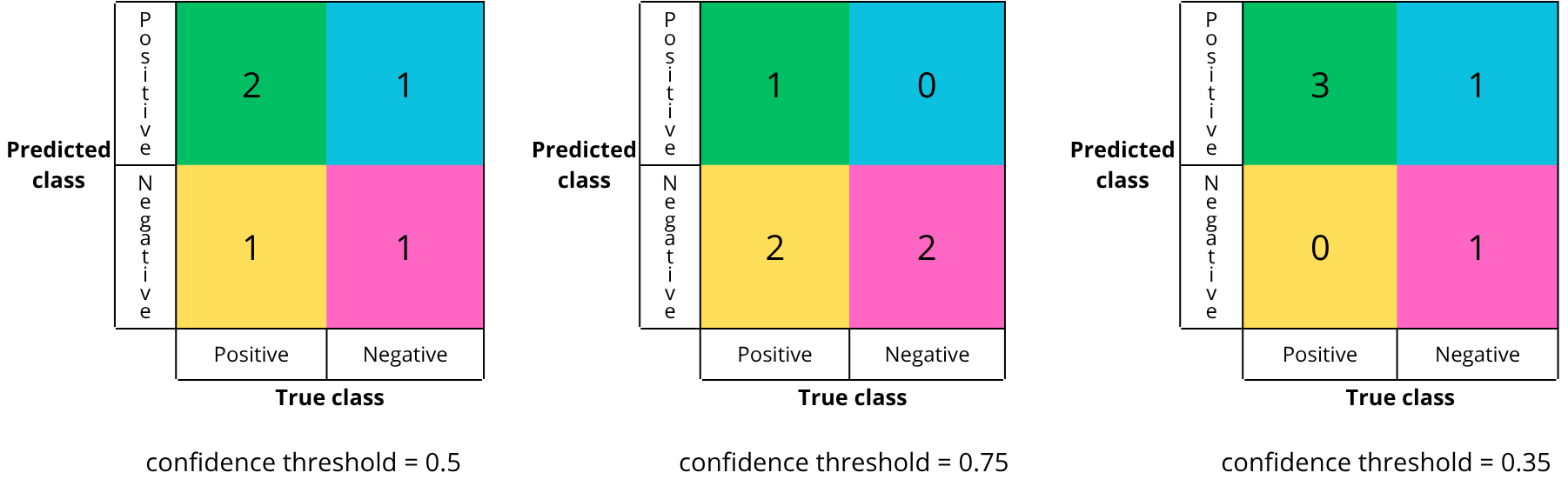
In theory, there are an infinite number of confusion matrices, as there are an infinite number of threshold values between 0 and 1.
The confusion matrix reflects the quality of the chosen confidence threshold. One key objective after training is to select the best threshold for deployment.
But how to know if a confusion matrix is a good one. A good matrix maximizes the correct diagonal (true positives and true negatives) and minimizes the bad diagonal (false positives and falses negatives).
However, in practice, reducing both errors simultaneously is difficult, so trade-offs must be made. For example, in medicine, false negatives are minimized (to avoid missing a disease), even if it increases false positives.
To determine the best threshold, we rely on evaluation metrics which we gonna see in the next section.