Section: Displot | Data Visualization on Seaborn

Section outline

The displot() function allows you to display different types of distributions.

signature displot

Parameter name	Description	Format	Example
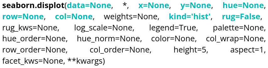
data	The dataframe you are working on	DataFrame, Series, dict, array, or list of arrays	data=table
x	Variable for the x-axis	String corresponding to a variable	x="weight"
y	Variable for the y-axis	String corresponding to a variable	y=”height”
hue	Allows to add a variable as different colors	String corresponding to a variable	hue=”age”
row	Allows to create a table of plots, controling the number of rows	String corresponding to a variable	row=”category”
col	Allows to create a table of plots, controling the number of columns	String corresponding to a variable	col=”job”
kind	Type of plot you want	String corresponding to a type	kind=”hist”,kind=”kde” ou kind=”ecdf”
rug	Allows to see individual data points on the axes	Boolean	rug=True

Here is an example code that creates a histogram:

data = sns.load_dataset("penguins")
sns.displot(data=data, x="bill_length_mm", rug=True, hue="sex", bins=20)
plt.show()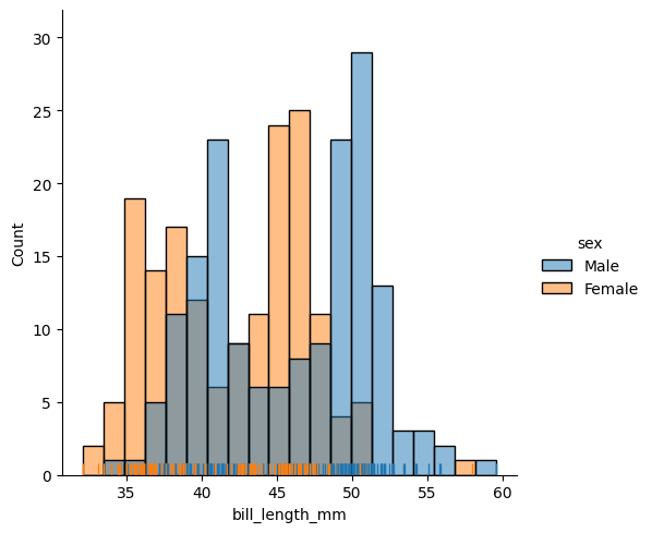

If you don’t specify the data for the y-axis, it will represent the number of occurrences, and if you don’t specify the kind, it defaults to a histogram. The bins argument controls the number of bars.

We also have access to kernel density estimation (KDE) to estimate a distribution. Here is an example of how to use it:

data = sns.load_dataset("penguins")
sns.displot(data=data,x="bill_length_mm", rug=True, hue="sex", kind="kde")
plt.show()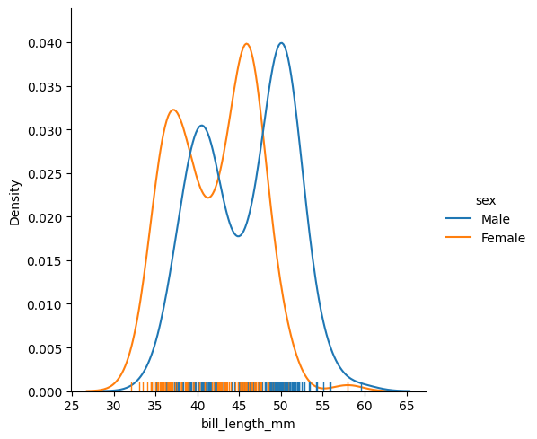

kde monodimensionnelle

If you specify a variable for the y-axis:

data = sns.load_dataset("penguins")
sns.displot(data=data,x="bill_length_mm", y="bill_depth_mm", rug=True, hue="sex", kind="kde")
plt.show()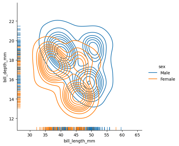

kde bidimensionnel

The rug parameter allows you to display individual observations along the axes of the plot.

The last type of distribution available is the ECDF (empirical cumulative distribution function). You cannot specify a y variable for this distribution since it is univariate.

data = sns.load_dataset("penguins")
sns.displot(data=data, x="body_mass_g", rug=True, hue="sex", kind="ecdf", row="species", col="sex", height=5)
plt.show()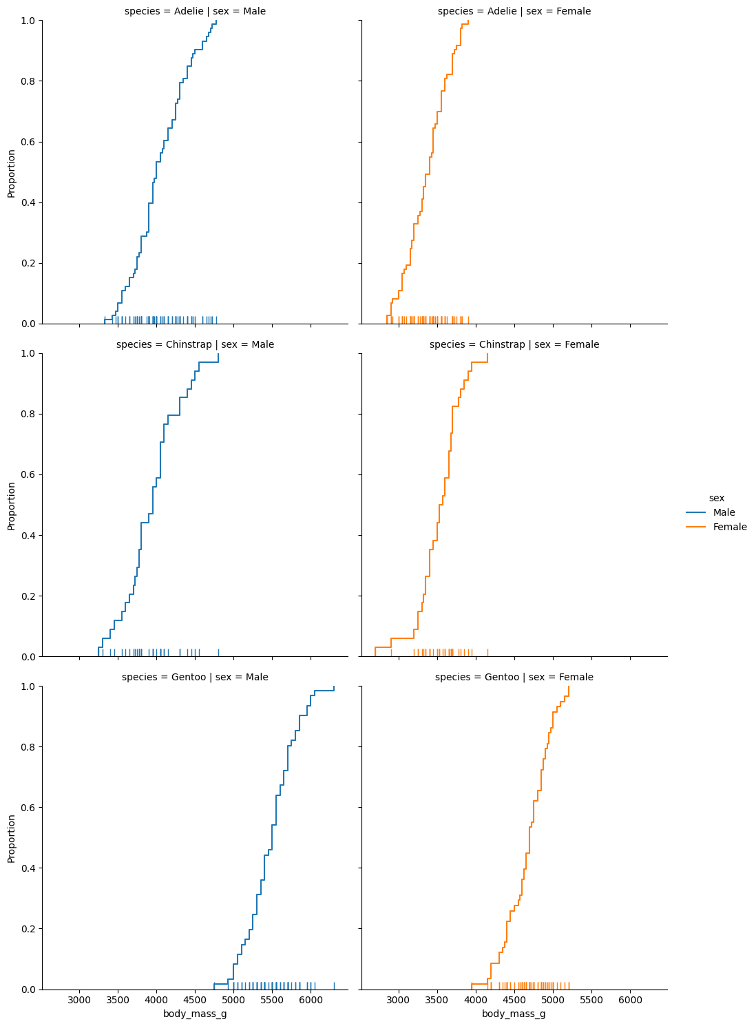

ecdf The row parameter allows you to display additional plots based on another variable in the dataset. The height parameter controls the height of the plots.